🔁 DDIM Inversion and Latent Space Manipulation

We explore the inversion and latent space manipulation of diffusion models, particularly the denoising diffusion implicit model (DDIM), a variant of the denoising diffusion probabilistic model (DDPM) with deterministic (and acceleratable) sampling and thus a meaningful mapping from the latent space \(\mathcal{Z}\) to the image space \(\mathcal{X}\). We implement and compare optimization-based, learning-based, and hybrid inversion methods adapted from GAN inversion, and we find that optimization-based methods work well, but learning-based and hybrid methods run into obstacles fundamental to diffusion models. We also perform latent space interpolation to show that the DDIM latent space is continuous and meaningful, just like that of GANs. Lastly, we apply GAN semantic feature editing methods to DDIMs, visualizing binary attribute decision boundaries to showcase the unique interpretability of the diffusion latent space.

Introduction

Latent spaces are a vital part of modern generative neural networks. Existing methods such as generative adversarial networks (GANs) and variational autoencoders (VAEs) all generate high-dimensional images from some low-dimensional latent space which encodes the features of the generated images. Thus, one can sample—randomly or via interpolation—this latent space to generate new images, and with the case of generative adversarial networks (GAN), at relatively high fidelity.

Since the latent space is, in a way, a low-dimensional representation of the generated images, we can model the generative network as a bijective function \(G : \mathcal{Z} \rightarrow \mathcal{X}\), where \(\mathcal{Z} \subseteq \mathbb{R}^d\) is the latent space and \(\mathcal{X} \subseteq \mathbb{R}^n\) is the image space, \(d \ll n\). Since the latent space encodes the most important visual features of the output images, to manipulate existing images, we can try to invert \(G\), \(G^{-1} : \mathcal{X} \rightarrow \mathcal{Z}\), to go from image space to latent space.

For VAEs, \(G^{-1}\) is trivially part of the architecture, but this is not the case for GANs and diffusion models. Luckily, GAN inversion is a very well-researched field. Although finding an analytical solution to \(G^{-1}\) is difficult, there are many ways to approximate the process, including

1. optimization-based methods, where we perform optimization to find the latent vector which best reconstructs the target image,
2. learning-based methods, where we train encoders that approximate \(G^{-1}\), and
3. hybrid methods, where we combine the two methods above, e.g., use learning-based methods to find a good initialization for optimization-based methods [2].

The logical next step is to directly apply the above methods directly to diffusion models—but there is a catch.

The Problem With Diffusion Models

The denoising diffusion probabilistic model (DDPM) is a relatively recent yet incredibly influential advancement in generative neural networks. Particularly, given an input image \(\mathbf{x}_0\) and some noise schedule \(\alpha_0, \alpha_1, \dots, \alpha_t\) (e.g., linear schedule) and \(\bar{\alpha}_t = \prod_{i = 1}^t \alpha_i\), it iteratively adds noise to the input image with increasing timesteps \(t \in \{ 1, 2, \dots, T \}\), described by

\[\mathbf{x}_t = \sqrt{\bar{\alpha}_t} \mathbf{x}_0 + \sqrt{1 - \bar{\alpha}_t} \boldsymbol{\epsilon} ,\]

where \(\boldsymbol{\epsilon} \sim \mathcal{N}(0, \mathbf{I})\) and \(T\) is the maximum timestep chosen so that \(\mathbf{x}_T\) resembles pure noise. Then, given some timestep \(t\), the network predicts the noise that was added from \(t - 1\) to \(t\). Formally, given the model \(\boldsymbol{\epsilon}_{\theta}\), we minimize

\[\mathcal{L}(\theta) = \left\| \boldsymbol{\epsilon} - \boldsymbol{\epsilon}_\theta (\mathbf{x}_t, t) \right\|^2 = \left\| \boldsymbol{\epsilon} - \boldsymbol{\epsilon}_\theta \left( \sqrt{\bar{\alpha}_t} \mathbf{x}_0 + \sqrt{1 - \bar{\alpha}_t} \boldsymbol{\epsilon}, t \right) \right\|^2\]

for some uniformly sampled time step \(t \sim \mathcal{U}(\{ 1, \dots, T \})\). Notice that, even though we heuristically add noise at every time \(t\), we can reparametrize that process as a single noise-adding step from \(\mathbf{x}_0\) to \(\mathbf{x}_t\), hence the use of \(\bar{\alpha}_t\) instead of \(\alpha_t\). To avoid effectively adding the same, unchanging noise \(\boldsymbol{\epsilon}\) at every time step, during sampling, we add small amounts of random noise every time the model subtracts the predicted noise from \(\mathbf{x}_t\) to get \(\mathbf{x}_{t - 1}\). Formally, starting with \(\mathbf{x}_T \sim \mathcal{N}(0, \mathbf{I})\), where \(\mathbf{x}_T \in \mathcal{Z}\), for \(t = T, \dots, 1\), we sample some \(\boldsymbol{\epsilon} \sim \mathcal{N}(0, \mathbf{I})\) every iteration if \(t > 1\), and we have

\[\mathbf{x}_{t - 1} = \frac{1}{\sqrt{\alpha_t}} \left( \mathbf{x}_t - \frac{1 - \alpha_t}{\sqrt{1 - \bar{\alpha}_t}} \boldsymbol{\epsilon}_\theta (\mathbf{x}_t, t) \right) + \sigma_t \boldsymbol{\epsilon} ,\]

where \(\sigma_t^2 = 1 - \alpha_t\), and we arrive at \(\mathbf{x}_0\), the generated image via denoising. Since we obtain \(\mathbf{x}_{t - 1}\) solely from \(\mathbf{x}_t\), the sampling process is a Markov chain.

Note that, unlike GANs, for diffusion models the latent space has the same dimensions as the image space, that is, \(\mathcal{Z}, \mathcal{X} \subseteq \mathbb{R}^n\).

The results of DDPMs are on-par with (and nowadays exceeding) GANs, and it has much greater stability in training as the generator is not trained via adversarial means [3] and thus is less prone to problems such as modal collapse, though it has the downside of a much longer sampling/generation time as it must make \(T\) forward passes through the model.

Naturally, we ask the question: can we invert DDPMs just like we can with GANs? In order for the above inversion methods to be applied to generative networks, we need two assumptions

1. the latent space maps to meaningful image features, and
2. the generator, i.e., \(G\), is deterministic.

Turns out, DDPMs does not satisfy the second assumption. Since the sampling process of DDPMs includes applying noise to the predicted \(\mathbf{x}_{t - 1}\) given \(\mathbf{x}_t\) for \(t > 0\), the generation process is not deterministic. Even if \(\mathcal{Z}\) does meaningfully map to \(\mathcal{X}\), latent space manipulation (without conditioning \(\boldsymbol{\epsilon}_\theta\), i.e., without providing it some additional semantic latent vector) cannot occur when the output image changes between different sampling passes, that is, \(G(\mathbf{z})\) is changes every execution even if \(\mathbf{z} \in \mathcal{Z}\) remains constant.

Moreover, optimization-based methods are computationally impractical for DDPMs, as since we are optimizing the reconstruction error of the generated image (compared to the target image) with respect to the (randomly initialized) latent vector, we must backpropagate through the entire Markovian sampling process with \(T\) iterations. (The standard value is \(T = 1000\), which is huge.) Not only is doing so very expensive, problems with extremely deep neural networks, such as gradient vanishing or explosion, begin to emerge.

Denoising Diffusion Implicit Models

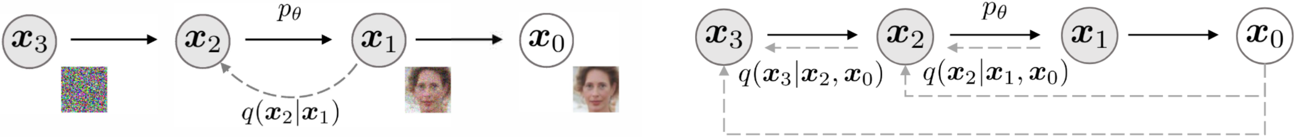
Figure 1: Illustrated comparison between diffusion (left) and non-Markovian (right) inference models. Crucially, we predict \(\mathbf{x}_{t - 1}\) with both \(\mathbf{x}_t\) and (predicted) \(\mathbf{x}_0\).

The denoising diffusion implicit model (DDIM) is a variation of the DDIM that, fundamentally, only modifies the inference/sampling step by making it non-Markovian. (In fact, Song et al. (2021) stated that pretrained DDPM models can even be used directly.) Particularly, it

1. has a deterministic sampling process, and
2. can accelerate sampling by taking timestep jumps larger than \(1\).

To do so, for notational simplicity, we rewrite \(\bar{\alpha}\) as \(\alpha\). Then, recall that we are optimizing

\[\mathcal{L}(\theta) = \left\| \boldsymbol{\epsilon} - \boldsymbol{\epsilon}_\theta (\mathbf{x}_t, t) \right\|^2 = \left\| \boldsymbol{\epsilon} - \boldsymbol{\epsilon}_\theta \left( \sqrt{\alpha_t} \mathbf{x}_0 + \sqrt{1 - \alpha_t} \boldsymbol{\epsilon}, t \right) \right\|^2 .\]

Notice that \(\boldsymbol{\epsilon}_\theta (\mathbf{x}_t, t)\) is not necessarily predicting the noise we added from \(\mathbf{x}_{t - 1}\) to \(\mathbf{x}_t\) but instead, due to the reparametrization to add the noise \(\boldsymbol{\epsilon}\) in one step, the noise we added from \(\mathbf{x}_0\)—the target image—to \(\mathbf{x}_t\). In other words, \(\boldsymbol{\epsilon}_\theta\) is separating the added noise \(\boldsymbol{\epsilon}\) from the original image \(\mathbf{x}_0 = \frac{1}{\sqrt{\alpha_t}} \left( \mathbf{x}_t - \sqrt{1 - \alpha_t} \boldsymbol{\epsilon} \right)\). We can also intuitively imagine how, the larger the \(t\), the less accurate the predicted target image

\[\hat{\mathbf{x}}_0 = \frac{1}{\sqrt{\alpha_t}} \left( \mathbf{x}_t - \sqrt{1 - \alpha_t} \boldsymbol{\epsilon}_\theta(\mathbf{x}_t, t) \right)\]

would be. Thus, during the inference process, given some \(\mathbf{x}_t\), instead of subtracting the predicted \(\boldsymbol{\epsilon}_\theta(\mathbf{x}_t, t)\) from \(\mathbf{x}_t\) to obtain \(\mathbf{x}_{t - 1}\), we can instead reconstruct \(\mathbf{x}_{t - 1}\) from the predicted \(\mathbf{x}_0\), \(\hat{\mathbf{x}}_0\), and the predicted noise \(\boldsymbol{\epsilon}_\theta(\mathbf{x}_t, t)\) both scaled with \(\alpha_t\)—like during training. Formally, accounting for the random noise \(\sigma_t \boldsymbol{\epsilon}\) we add in DDPMs, we have

\[\mathbf{x}_{t - 1} = \sqrt{\alpha_{t - 1}} \underbrace{\left( \frac{\mathbf{x}_t - \sqrt{1 - \alpha_t} \boldsymbol{\epsilon}_\theta(\mathbf{x}_t, t)}{\sqrt{\alpha_t}} \right)}_{\textrm{predicted } \mathbf{x}_0 \textrm{, i.e., } \hat{\mathbf{x}}_0} + \sqrt{1 - \alpha_{t - 1} - \sigma_t^2} \underbrace{\boldsymbol{\epsilon}_\theta(\mathbf{x}_t, t)}_{\textrm{added noise}} + \underbrace{\sigma_t \boldsymbol{\epsilon}}_{\textrm{random noise}} ,\]

where we define \(\alpha_0 = 1\). Crucially, different choices of \(\sigma_t\) results in different generative processes despite the training objective and resulting model \(\boldsymbol{\epsilon}_\theta\) remaining the same. Particularly, when \(\sigma_t = \sqrt{\frac{1 - \alpha_{t - 1}}{1 - \alpha_t}} \sqrt{1 - \frac{\alpha_t}{\alpha_{t - 1}}}\) (in this more complex form because we rewrote \(\bar{\alpha}\) as \(\alpha\)), the process is Markovian and becomes equivalent to the DDPM. On the other hand, when \(\sigma_t = 0\) for all \(t \in \{ 1, \dots, T \}\), the sampling process becomes deterministic as we are no longer adding random noise every iteration. Therefore, as Song et al. (2021) claims, the model becomes an implicit probabilistic model, thus the name denoising diffusion implicit model (DDIM). Since now we are mirroring the forward process in the sampling process, where \(\mathbf{x}_t\) could depend on both \(\mathbf{x}_0\) and \(\mathbf{x}_{t - 1}\), the inference step is non-Markovian.

Moreover, since we have the predicted \(\mathbf{x}_0\) and \(\boldsymbol{\epsilon}\), we can use them to reconstruct any timestep of \(\mathbf{x}\). Particularly, we can write

\[\mathbf{x}_{t - \Delta t} = \sqrt{\alpha_{t - \Delta t}} \left( \frac{\mathbf{x}_t - \sqrt{1 - \alpha_t} \boldsymbol{\epsilon}_\theta(\mathbf{x}_t, t)}{\sqrt{\alpha_t}} \right) + \sqrt{1 - \alpha_{t - \Delta t}} \boldsymbol{\epsilon}_\theta(\mathbf{x}_t, t)\]

for any \(\Delta t \leq t\), where we can drastically accelerate the inference process by setting \(\Delta t \gg 1\). Doing so makes optimization-based inversion methods possible for large \(\Delta t\). In practice, DDIMs tend to have slightly worse generation quality than DDPMs, especially with \(\Delta t \gg 1\), mostly in the decrease in texture and detail [1].

In summary, DDIMs address the problems with DDPMs by making the sampling process deterministic and fast. Therefore, with that foundation, we aim to apply GAN inversion methods to DDIMs and explore if we can reverse the diffusion process.

Implementing DDIMs

We closely follow the original PyTorch implementation of the DDIM [1] with some slight modifications to account for the much reduced network sizes (due to computational limits) inspired by [2]. All models are trained and tuned from scratch as the pretrained models are generally too large for optimization-based methods.

Notably, we will be training everything from scratch and not using any pre-trained models. Many diffusion-based generative models today are incredibly massive and impractical to train and test on single computers, so we also want to explore training smaller networks.

Data

We train DDIMs on several datasets, including

• CelebA: Large-scale CelebFaces Attributes Dataset,
• FFHQ: Flickr-Faces-HQ Dataset,
• LSUN Churches: Construction of a Large-scale Image Dataset using Deep Learning with Humans in the Loop, church_outdoor class,
• Flowers102: 102 Category Flower Dataset,
• ImageNet: ImageNet Large-scale Visual Recognition Challenge,
• Miniplaces: Provided by Professor Bolei Zhou for his COM SCI 188 course (Winter 2023), a subset of Places365, and
• Anime Faces: A Kaggle dataset of anime faces.

We normalize all data to \([-1, 1]\) and perform random horizontal flip as the only data augmentation.

Network

For our neural network \(\boldsymbol{\epsilon}_\theta\), we use the model design heuristic of DDPMs, that is, a denoising U-Net (i.e., matching input and output sizes), with additional self-attention blocks at the \(16 \times 16\) resolution between the convolutional blocks.

A lot of code below takes inspiration from [1C], though we do make many structural changes that fit the repository better.

Time Embeddings

We use time embeddings from the original “Attention is All You Need” paper.

def time_embed(t, embed_dim):
    half_dim = embed_dim // 2
    exp_factor = np.log(10000) / (half_dim - 1)
    embed = torch.exp(torch.arange(half_dim, dtype=torch.float32).mul(-exp_factor))
    embed = embed.to(t.device)  # Move embeddings to GPU (if possible)
    embed = t.to(torch.float32)[:, None] * embed[None, :]  # Pair-wise multiplication
    embed = torch.cat([torch.sin(embed), torch.cos(embed)], dim=1)
    if embed_dim % 2 == 1:  # Zero padding if embed_dim is odd
        embed = F.pad(embed, (0, 1, 0, 0))
    return embed

Residual Blocks

We employ residual blocks with two convolutions, group normalization, optional dropout, and optional \(3 \times 3\) convolutions for skip connections of mistmatching input and output channels (\(1 \times 1\) is the default for the ResNet). Each residual block also takes sinusoidal time embeddings and projects it through a linear layer to be summed with the feature map from the first convolution, as ‘time’ (i.e., \(t\) in \(\mathbf{x}_t\)) is an extremely important indicator for noise. We use \(\textrm{Swish}\) as the activation function.

During testing we found that replacing group normalization for batch normalization in small networks can work better for enhancing detail at the cost of global coherence, which may be beneficial for datasets like Flowers102. Thus, for the group_norm function we added the option to set num_groups=-1 that defaults to batch normalization.

class ResnetBlock(nn.Module):

    def __init__(self, in_channels, out_channels=None, do_conv_skip=False,
                 dropout=0.0, time_embed_channels=128, num_groups=16):
        super().__init__()
        self.in_channels = in_channels
        out_channels = in_channels if out_channels is None else out_channels
        self.out_channels = out_channels

        # Convolution layer 1
        self.norm_1 = nutils.group_norm(in_channels, num_groups=num_groups)
        self.conv_1 = nn.Conv2d(in_channels, out_channels, kernel_size=3, stride=1, padding=1)
        self.time_embed_proj = nn.Linear(time_embed_channels, out_channels)
        # Convolution layer 2
        self.norm_2 = nutils.group_norm(out_channels, num_groups=num_groups)
        self.dropout = nn.Dropout(dropout)
        self.conv_2 = nn.Conv2d(out_channels, out_channels, kernel_size=3, stride=1, padding=1)
        # ResNet skip layer (with 3x3 kernel option available with do_conv_skip)
        if in_channels != out_channels:
            kernel_size = 3 if do_conv_skip else 1  # Skip with larger kernel
            self.conv_skip = nn.Conv2d(in_channels, out_channels, kernel_size=kernel_size,
                                       stride=1, padding=kernel_size // 2)

    def forward(self, x, time_embed):
        h = x  # Order for each layer: norm -> activation -> conv
        h = self.norm_1(h)
        h = nutils.swish(h)
        h = self.conv_1(h)

        time_embed = nutils.swish(time_embed)
        h = h + self.time_embed_proj(time_embed)[:, :, None, None]  # Apply to each channel

        h = self.norm_2(h)
        h = nutils.swish(h)
        h = self.dropout(h)  # Apply dropout on second convolution layer
        h = self.conv_2(h)

        if self.in_channels != self.out_channels:
            x = self.conv_skip(x)

        h = x + h
        return h

Attention Blocks

At the \(16 \times 16\) resolution level, we apply a convolution self-attention block with a skip connection. We also apply self-attention between the two residual blocks in the middle of the U-Net. Notice that, since we set kernel_size=1 and stride=1 for the \(Q\), \(K\), and \(V\) convolutions, we essentially have an element-wise linear layer with weights shared across each entry on the feature map (across channels).

class AttentionBlock(nn.Module):

    def __init__(self, in_channels, num_groups=32):
        super().__init__()

        self.norm = nutils.group_norm(in_channels, num_groups=num_groups)
        self.Q = nn.Conv2d(in_channels, in_channels, kernel_size=1, stride=1, padding=0)
        self.K = nn.Conv2d(in_channels, in_channels, kernel_size=1, stride=1, padding=0)
        self.V = nn.Conv2d(in_channels, in_channels, kernel_size=1, stride=1, padding=0)
        self.out_proj = nn.Conv2d(in_channels, in_channels, kernel_size=1, stride=1, padding=0)

    def forward(self, x):
        h = x
        h = self.norm(h)
        q = self.Q(h)
        k = self.K(h)
        v = self.V(h)

        # Compute attention
        B, C, H, W = q.shape
        q = q.reshape(B, C, H * W).moveaxis(-1, -2)  # B C H W -> B (H W) C
        k = k.reshape(B, C, H * W)  # B C H W -> B C (H W)
        w = q @ k  # Batched scores, B (H W) (H W), w[b, i, j] = sum_c q[b, i, c] k[b, c, j]
        w.mul_(pow(C, -0.5))  # Normalize scores
        w = F.softmax(w, dim=-1)  # Apply softmax in preparation for summing

        # Apply attention to values
        v = v.reshape(B, C, H * W)  # B C H W -> B C (H W)
        w = w.moveaxis(-1, -2)  # B (H W of q) (H W of k) -> B (H W of k) (H W of q)
        h = v @ w  # Batched attention, B C (H W) (H W of q), sum_i v[b, c, i] w[b, i, j]
        h = h.reshape(B, C, H, W)  # ^ Taking linear combination of values weighted by cores

        h = self.out_proj(h)
        h = x + h  # Residual skip connection
        return h

U-Net

The U-Net architecture is similar to that of the PixelCNN++, with the addition of the attention layers mentioned above. Particularly, we employ long skip connections between every pair of residual blocks (one in the downsampling layers and one in the mirroring upsampling layers). Each resolution level has num_blocks number of residual blocks before down/upsampling (usually num_blocks=2). Note that we do not include the code for the classes Downsample and Upsample here, but they are merely linearly-interpolated down/upsampling layers with optional \(3 \times 3\) convolutions afterwards.

Additionally, we initialize the final output convolution layer with zeros, as inspired by [2C]. This improves the stability of the first few iterations as now it begins by predicting zeros, i.e., the mean of the noise prediction as \(\boldsymbol{\epsilon} \sim \mathcal{N}(0, \mathbf{I})\), so the loss begins at (approximately) \(1\).

class UNet(nn.Module):

    def __init__(self, in_shape, hidden_channels, num_blocks, channel_mults, attention_sizes,
                 time_embed_channels, dropout=0.0, num_groups=16, do_conv_sample=True):
        super().__init__()

        assert in_shape[1] == in_shape[2], f"Input shape must be square."

        self.in_shape = in_shape
        self.hidden_channels = hidden_channels
        self.num_sizes = len(channel_mults)
        self.num_blocks = num_blocks

        # Time embedding

        self.time_embed = nn.Module()
        self.time_embed.fn = partial(nutils.time_embed, embed_dim=hidden_channels)
        self.time_embed.dense = nn.ModuleList([
            nn.Linear(hidden_channels, time_embed_channels),
            nn.Linear(time_embed_channels, time_embed_channels)])

        # Downsampling layers

        self.in_conv = nn.Conv2d(in_shape[0], hidden_channels, kernel_size=3, stride=1, padding=1)

        current_size = in_shape[1]
        in_channel_mults = [1] + channel_mults
        self.down_layers = nn.ModuleList()
        in_channels_block = None
        for i in range(len(channel_mults)):
            blocks = nn.ModuleList()
            attentions = nn.ModuleList()
            in_channels_block = round(hidden_channels * in_channel_mults[i])
            out_channels_block = round(hidden_channels * channel_mults[i])
            # Add num_blocks Resnet blocks (with Attention blocks)
            for _ in range(num_blocks):
                blocks.append(ResnetBlock(in_channels_block, out_channels_block,
                                          time_embed_channels=time_embed_channels,
                                          dropout=dropout, num_groups=num_groups))
                in_channels_block = out_channels_block
                if current_size in attention_sizes:
                    attentions.append(AttentionBlock(in_channels_block, num_groups=num_groups))
            # Create down layer as nn.Module
            down_layer = nn.Module()
            down_layer.blocks = blocks
            down_layer.attentions = attentions
            if i != len(channel_mults) - 1:  # Downsample unless at last layer
                down_layer.downsample = Downsample(in_channels_block, do_conv=do_conv_sample)
                current_size = current_size // 2
            self.down_layers.append(down_layer)

        # Middle layers

        self.mid_layers = nn.ModuleList()
        self.mid_layers.block_1 = ResnetBlock(in_channels_block, in_channels_block,
                                              time_embed_channels=time_embed_channels,
                                              dropout=dropout, num_groups=num_groups)
        self.mid_layers.attention = AttentionBlock(in_channels_block, num_groups=num_groups)
        self.mid_layers.block_2 = ResnetBlock(in_channels_block, in_channels_block,
                                              time_embed_channels=time_embed_channels,
                                              dropout=dropout, num_groups=num_groups)

        # Upsampling layers

        self.up_layers = nn.ModuleList()
        for i in reversed(range(len(channel_mults))):
            blocks = nn.ModuleList()
            attentions = nn.ModuleList()
            out_channels_block = round(hidden_channels * channel_mults[i])
            in_channels_skip = round(hidden_channels * channel_mults[i])
            for j in range(num_blocks + 1):
                if j == num_blocks:
                    in_channels_skip = hidden_channels * in_channel_mults[i]
                blocks.append(ResnetBlock(in_channels_block + in_channels_skip, out_channels_block,
                                          time_embed_channels=time_embed_channels,
                                          dropout=dropout, num_groups=num_groups))
                in_channels_block = out_channels_block
                if current_size in attention_sizes:
                    attentions.append(AttentionBlock(in_channels_block, num_groups=num_groups))
            # Create up layer as nn.Module
            up_layer = nn.Module()
            up_layer.blocks = blocks
            up_layer.attentions = attentions
            if i != 0:
                up_layer.upsample = Upsample(in_channels_block, do_conv=do_conv_sample)
                current_size *= 2
            self.up_layers.insert(0, up_layer)

        # End layers

        self.out_norm = nutils.group_norm(in_channels_block, num_groups=num_groups)
        self.out_conv = nn.Conv2d(in_channels_block, in_shape[0],
                                  kernel_size=3, stride=1, padding=1)
        self.out_conv.weight.data.fill_(0.0)

    def forward(self, x, t):
        assert list(x.shape[-3:]) == self.in_shape, \
               f"Shape of x {tuple(x.shape)} does not match network definition."

        # Time embedding
        t_embed = self.time_embed.fn(t)
        t_embed = self.time_embed.dense[0](t_embed)
        t_embed = nutils.swish(t_embed)
        t_embed = self.time_embed.dense[1](t_embed)

        # Downsampling

        h_skip = [self.in_conv(x)]
        for i in range(self.num_sizes):
            for j in range(self.num_blocks):
                h = self.down_layers[i].blocks[j](h_skip[-1], t_embed)
                if len(self.down_layers[i].attentions) > 0:  # Apply attention heads
                    h = self.down_layers[i].attentions[j](h)
                h_skip.append(h)
            if i != self.num_sizes - 1:
                h = self.down_layers[i].downsample(h_skip[-1])
                h_skip.append(h)

        # Middle

        h = h_skip[-1]
        h = self.mid_layers.block_1(h, t_embed)
        h = self.mid_layers.attention(h)
        h = self.mid_layers.block_2(h, t_embed)

        # Upsampling

        for i in reversed(range(self.num_sizes)):
            for j in range(self.num_blocks + 1):
                h = torch.cat([h, h_skip.pop()], dim=-3)  # Concatenate with skip at channel
                h = self.up_layers[i].blocks[j](h, t_embed)
                if len(self.up_layers[i].attentions) > 0:  # Apply attention heads
                    h = self.up_layers[i].attentions[j](h)
            if i != 0:
                h = self.up_layers[i].upsample(h)

        # End

        h = self.out_norm(h)
        h = nutils.swish(h)
        h = self.out_conv(h)
        return h

Diffusion

We follow the training and inference processes as defined by the original DDPM and DDIM paper. Particularly, we use the code structure from [3C] and the methods from [1C]. Many of the code snippets presented below are within the Diffusion runner class.

Forward Process

The noise-adding function, or q_sample from the forward process \(q(\mathbf{x}_t \mid \mathbf{x}_{t - 1}, \, \mathbf{x}_0)\) as described in [1], adds the scheduled noise by first computing \(\alpha_t\) and then passing the noisy inputs through the network \(\boldsymbol{\epsilon}_\theta\) to obtain the predicted noise.

def q_sample(self, x_0, t, e):
    """
    We express x_t as a linear combination of x_0 and noise e because
        q(x_t | x_0) = N(x_t; sqrt(a_t) x_0, (1 - a_t) I) .
    This is the key difference between DDPM and DDIM. The former tries to approximate e where
        x_(t - 1) + e = x_t ,
    whereas the latter mixes e and x_0 via a_t (see above). Because we are now using x_0, this
    is no longer a Markov chain, and during the p_sample process we can speed up the sampling
    process by skipping an arbitrary number of t each time just by parameterizing a_t.

    For more information: https://strikingloo.github.io/wiki/ddim
    """
    b = self.betas
    with torch.no_grad():
        a_t = (1.0 - b).cumprod(dim=0).index_select(dim=0, index=t)[:, None, None, None]
        x_t = a_t.sqrt() * x_0 + (1.0 - a_t).sqrt() * e  # DDIM Eq. 4
    output = self.network(x_t, t=t.to(torch.float32))  # Predicted e
    return output

Training

The training function calls q_sample and computes the error between the predicted noise and added noise. Notably, even though both the DDPM and DDIM paper defines the error as the \(L_2\) distance between the output \(\boldsymbol{\epsilon}_\theta(\mathbf{x}_t, t)\) and added noise \(\boldsymbol{\epsilon}\), in practice we found, for much fewer training iterations, using \(L_1\) distance as the loss function both improves detail and reduces artifacts. Thus, we use \(L_1\) loss, i.e., mean absolute error, instead.

Interestingly, with smaller models, \(L_2\) loss actually causes bad colorcasting, especially during earlier iterations, whereas \(L_1\) loss does not.

The below is an abridged version of the code that removes all the auxiliary elements not directly relevant to the training logic, e.g., dataset/loader initialization, optimizer, exponential moving average (EMA), tqdm, TensorBoard, model checkpoint saving, etc. To see details of auxiliary code, check the linked official code repository of this project.

def train(self):
    config = self.config

    train_loader =  # Initialize PyTorch training loader with data

    network = self.network

    optimizer =  # Initialie optimizer (usually Adam)

    i = 0
    while i < config.training.num_i:
        for _, (x_0, _) in enumerate(train_loader):

            n = x_0.shape[0]
            network.train()

            x_0 = x_0.to(self.device)
            x_0 = self.data_transform(x_0)
            e = torch.randn_like(x_0)  # Noise to mix with x_0 to create x_t

            # Arithmetic sampling
            t = torch.randint(low=0, high=config.diffusion.num_t, size=(n // 2 + 1,),
                              device=self.device)
            t = torch.cat((t, config.diffusion.num_t - t - 1), dim=0)[:n]
            output = self.q_sample(x_0=x_0, t=t, e=e)  # Estimate noise added
            loss = rutils.criterion(output, e, name=config.training.criterion)

            optimizer.zero_grad()
            loss.backward()

            try:  # Perform gradient clipping only if defined in config
                nn.utils.clip_grad_norm_(network.parameters(), config.optimizer.gradient_clip)
            except AttributeError:
                pass
            optimizer.step()

            i += 1
            if i >= config.training.num_i:  # Training for exactly num_i iterations
                break

Sampling

The sampling function is the same as described above in the introduction. Note that we add the option to return the entire generation sequence, including the progressively denoised \(\mathbf{x}_t\) and \(\mathbf{x}_0\) predictions computed from the network’s noise prediction. We also removed some auxiliary code elements here to focus on the sampling algorithm itself.

def p_sample(self, x, network=None, num_t=None, num_t_steps=None, skip_type="uniform",
             eta=None, ema=True, sequence=False):
    config = self.config

    network = utils.get_default(network, default=self.network)
    network.eval()

    if skip_type == "uniform":
        t_skip = num_t // num_t_steps
        t_sequence = list(range(0, num_t, t_skip))
    elif skip_type == "quadratic":
        t_sequence = np.square(np.linspace(0, np.sqrt(0.8 * num_t), num_t_steps))
        t_sequence = [int(t) for t in t_sequence]
    else:
        raise NotImplementedError(f"Time skip type {skip_type} not supported.")

    n = x.shape[0]
    b = self.betas
    t_sequence_next = [-1] + t_sequence[:-1]
    x_0_predictions = []
    x_t_predictions = [x]

    for i, j in zip(reversed(t_sequence), reversed(t_sequence_next)):
        t = (torch.ones(n) * i).to(self.device)  # Same time across batch
        t_next = (torch.ones(n) * j).to(self.device)

        a_t = rutils.alpha(b=b, t=t)
        a_t_next = rutils.alpha(b=b, t=t_next)

        x_t = x_t_predictions[-1]
        e_t = network(x_t, t=t)

        x_0_t = (x_t - (1.0 - a_t).sqrt() * e_t) / a_t.sqrt()  # DDIM Eq. 12, "predicted x_0"
        x_0_predictions.append(x_0_t.detach().cpu())

        # DDIM Eq. 16, s_t is constant for amount of random noise during generation.
        # If eta == 0, then we have DDIM; if eta == 1, then we have DDPM
        s_t = eta * (((1.0 - a_t_next) / (1.0 - a_t)) * ((1.0 - a_t) / a_t_next)).sqrt()
        e = s_t * torch.randn_like(x)  # DDIM Eq. 12, "random noise"

        # DDIM Eq. 12, "direction pointing to x_t"
        x_d = ((1.0 - a_t_next) - s_t.square()).sqrt() * e_t

        x_t_next = a_t_next.sqrt() * x_0_t + x_d + e  # DDIM Eq. 12
        x_t_predictions.append(x_t_next)  # Only keep gradients of final x_t prediction
        x_t_predictions[-2] = x_t_predictions[-2].detach().cpu()

    if not sequence:  # Only return final generated images
        return x_t_predictions[-1]
    return x_t_predictions, x_0_predictions  # Return entire generation process

Inversion

Optimization-based Method

Heuristically, optimization-based methods are the simplest. Particularly, we implement the gradient-based method. Given some image \(\mathbf{x}\), we are minimizing

\[\mathcal{L}(\mathbf{z}) = \mathcal{R}(G(\mathbf{z}), \mathbf{x}) ,\]

where \(G\) is the short hand (“generator”) for the full DDIM inference process and \(\mathcal{R}\) is the reconstruction loss and can include

• \(L_1\) loss, where \(\mathcal{R}(\hat{\mathbf{x}}, \mathbf{x}) = \frac{1}{n} \sum_{i} \lvert \mathbf{x}_i - \hat{\mathbf{x}}_i \rvert\),
• \(L_2\) loss, where \(\mathcal{R}(\hat{\mathbf{x}}, \mathbf{x}) = \frac{1}{n} \sum_{i} (\mathbf{x}_i - \hat{\mathbf{x}}_i)^2\),
• \(L_\infty\) loss, where \(\mathcal{R}(\hat{\mathbf{x}}, \mathbf{x}) = \lvert \mathbf{x}_j - \hat{\mathbf{x}}_j \rvert\) where \(j = \max_i \lvert \mathbf{x}_i - \hat{\mathbf{x}}_i \rvert\),
• peak signal-to-noise ratio (PSNR), where \(\mathcal{R}(\hat{\mathbf{x}}, \mathbf{x}) = 10 \log_{10} \left( \frac{\textrm{MAX}^2}{\textrm{MSE}} \right)\), where \(\textrm{MAX}\) is the maximum possible value of the image (i.e., \(1\)) and \(\textrm{MSE}\) is the \(L_2\) loss, and
• structural similarity (SSIM), which is more complex to typeset and does not perform that well, so I will merely leave a link to more information about it instead [2].

Note that, for PSNR and SSIM, unlike \(L_p\) losses, the higher the value, the better the reconstruction, so we instead maximize \(\mathcal{L}\) in those cases.

With the loss function defined, we can simply perform optimization (e.g., SGD, Adam, etc.) with the gradient \(\frac{\partial \mathcal{L}}{\mathbf{z}}\), iteratively updating \(\mathbf{z}\) until convergence, at which point \(\hat{\mathbf{x}} = G(\mathbf{z})\) should be a good reconstruction of \(\mathbf{x}\).

Note that gradient-based methods are really only computationally viable with DDIMs, as we can set \(\Delta t\) to be large so the gradients do not have to propagate through much fewer passes of the network. Even with this optimization-based methods can be quite slow compared to learning-based methods.

def gradient_inversion(z=None, target=None, diffusion=None, lr=0.01, num_i=100, num_t_steps=10,
                       criterion="l1"):
    device = diffusion.device

    z = utils.get_default(z, default=torch.randn(*target.shape, device=device))
    if target is None or diffusion is None:
        return z
    z.requires_grad_()

    maximize = criterion in ["psnr", "ssim"]
    optimizer = optim.Adam([z], lr=lr, betas=(0.9, 0.999), eps=1e-8, maximize=maximize)
    target = target.to(device)

    for _ in range(num_i):
        y = diffusion.sample(x=z, sequence=False, ema=True, num_t_steps=num_t_steps)[0]
        loss = rutils.criterion(y, target, name=criterion)
        loss.backward()
        optimizer.step()
        optimizer.zero_grad()

    return z

Learning-based Method

We experimented with learning-based methods with two types of objectives. Suppose we have an encoder \(E : \mathcal{X} \rightarrow \mathcal{Z}\) that maps some input image \(\mathbf{x} \in \mathcal{X}\) to its corresponding noise latent \(\mathbf{z} \in \mathcal{Z}\) such that \(G(\mathbf{z}) \approxi \mathbf{x}\). Then, we can either

1. minimize \(\mathcal{R}(E(\mathbf{x}), \mathbf{z})\), i.e., minimizing the error within the latent space, and
2. minimize \(\mathcal{R}(G(E(\mathbf{x})), \mathbf{x})\), i.e., minimizing the error within the image space (reconstruction loss),

where \(\mathcal{R}\) can be any loss between two vectors such as \(L_2\) as mentioned in the previous subsubsection. We do not show results for both these methods as they do not work well at all, at least with the rough implementation we have in our code base, which is linked at the very top of this article. We discuss why this is the case in the Results section below.

Hybrid Method

Because, as mentioned, the learning-based method does not work well, at least with our rudimentary implementation, we do not explore the hybrid method. Particularly, since the hybrid method uses some learning-based method as a noise initializer and then some optimization-based method to finetune the noise, if the noise initializer is not great to begin with, there is not much point to the hybrid method.

Semantic Feature Editing

Suppose we get good results from optimization-based inversion and interpolation (explored later). Then, we know this indicates that the DDIM, and more generally, diffusion models with deterministic inference, does have a one-to-one mapping between the noise latent space \(\mathcal{Z}\) and image space \(\mathcal{X}\) that is continuously ‘meaningful.’ Since learning-based (and consequently hybrid-based) methods did not work, we explore another technique for manipulating the latent space of generative models, particularly GANs. Specifically, we replicate parts of [4] with the DDIM.

Suppose we generate many noise-image pairs with our trained DDIM, so \(\mathbf{z}\) and its corresponding \(\mathbf{x} = G(\mathbf{z})\). Also, suppose that our original dataset has additional labels for each image in the dataset which correspond to binary features such as age, eyeglasses, masculinity. Then, we can do the following.

1. First, train a multinomial classifier that can label these images with their corresponding binary attributes.
2. Then, with each \(\mathbf{x}\), find its corresponding binary attributes with the trained classifier. Suppose the resulting attributes are \(f_1, \dots, f_m\) for \(m\) multinomial classes.
3. Then, for any specific binary feature \(f_i\), we train a binary classifier \(\mathbf{w}^T \mathbf{z} + b = \hat{f}_i\) that finds a hyperplane in the noise latent space (which we can do as the \(\mathbf{z}\) and \(\mathbf{x}\) are paired) which separates the positive and negative instances of the chosen binary attribute.

Notice that said hyperplane, when translated to contain the origin, is exactly described by \(\mathbf{w}\), as we compute points on a hyperplane with \(\mathbf{n} \cdot \mathbf{x} = \mathbf{n}^T \mathbf{x}\), where \(\mathbf{n}\) is the normal vector of the hyperplane. Importantly, \(\mathbf{w}\)—the weights of the binary classifier—is exactly the normal vector of the hyperplane. In other words, \(\mathbf{w}\) describes the direction to nudge/push the noise latent \(\mathbf{z}\) that maximizes the binary feature \(f_i\), and correspondingly \(-\mathbf{w}\) describes the direction that minimizes said binary feature. To ensure that the ‘amount’ in which we nudge by \(\mathbf{w}\) is consistent across different binary classifier instances, we normalize the direction vector with \(\mathbf{u} = \frac{1}{\| \mathbf{w} \|} \mathbf{w}\). Therefore, by modifying \(\mathbf{z}\) with

\[\mathbf{z}' = \mathbf{z} + \alpha \mathbf{u}\]

for some \(\alpha \in \mathbb{R}\), we can semantically edit attributes/features of the paired image \(\mathbf{x}\) when we compute \(\mathbf{x}' = G(\mathbf{z}')\).

Results

DDIM Generation

Figure 2: Sample generated images with DDIM, with the final generated results (left) and evolution of some fixed latent over the training process with EMA parameters (right). We generate the samples with num_t_step=50. The datasets used, from the top to bottom, are CelebA, FFHQ, LSUN Churches, Flowers102, ImageNet, Miniplaces, and Anime Faces.

We train DDIMs on the datasets CelebA, FFHQ, LSUN Churches, Flowers102, ImageNet, Miniplaces, and Anime Faces with identical architectures as the output images are all \(64 \times 64\). Particularly, we set filters of \([128, 256, 256, 256, 512]\) with self-attention at the \(16 \times 16\) resolution (so right after the second \(256\) layer), with each filter layer consisting of two residual blocks and then a down/upsampling module. We select \(128\) as the time embedding dimensions. We set a dropout of \(0.1\). We use \(3 \times 3\) convolutions for mismatching channel residual skips, and we also use \(3 \times 3\) convolutions (after interpolation) for down/upsampling. The model is about \(75.3\) million parameters. We did find significant generation quality improvements of the \(75\)-million model compared to much smaller \(5\)- to \(10\)-million parameter models, especially for LSUN Churches and Miniplaces.

Following DDPM and DDIM, we set \(T = 1000\), \(\beta_1 = 0.0001\), and \(\beta_T = 0.02\) (\(\alpha_t = 1 - \beta_t\), here \(\alpha\) is notated as it is in DDPM, for DDIM we need to take the cumulative product as well), with a default sampling step of \(50\), so \(\Delta t = \frac{1000}{50 - 1}\). \(\sigma_t = 0\) for all \(t \in \{ 1, \dots, T \}\) for deterministic sampling.

We use the Adam optimizer with learning rate \(0.0002\) and default hyperparameters for \(72000\) iterations with a batch size of \(64\). Doing so takes approximately \(11\) hours on a single 450W NVIDIA RTX 3090Ti with 24GB VRAM. We also clip the gradient entries to \(1.0\) to improve model stability. We also set an EMA of \(0.9995\) for the model parameters to further improve stability, which is less than DDPM and DDIM’s \(0.9999\) as they train for much more iterations. We do not use weight decay, as we found doing so decreases the output generation quality.

Inversion

Optimization-based Method

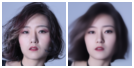
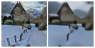
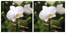
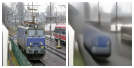
Figure 3: Inversion with optimization-based method (using Adam optimizer), with the original image \(\mathbf{x}\) (left), reconstructed image \(\hat{\mathbf{x}}\) (middle), and evolution of the reconstruction during training (right). The reconstructed PSNR is generally around \(23 \textrm{dB}\) to \(29 \textrm{dB}\).

We use the Adam optimizer with learning rate \(0.01\) and maximize PSNR loss. We set \(\Delta t = \frac{1000}{10 - 1}\) (i.e., num_t_steps=10) and optimize for \(300\) iterations. The initial latent vector \(\mathbf{z}\) is randomly initialized.

Notice that the optimization-based method generally reconstructs the global features of the image but can be lacking in fine detail, which can be partly attributed to the small num_t_steps (i.e., large \(\Delta t\)) since increasing it generally leads to longer inversion time (as we need to backpropagate through more passes of the network), larger number of iterations (gradient vanishing starts to occur with more backpropagations), and more complex loss landscapes (i.e., a more difficult optimizationt task).

Note that the images we test inversion on are all in the validation split of their respective datasets, that is, the images are not used to train the model.

Learning-based Method

Figure 4: Inversion reconstruction examples with learning-based methods of option 1 (noise latent error, left) and option 2 (reconstruction error, right) after training the encoder for \(\sim 10000\) iterations.

As mentioned in the Methods section, the learning-based method does not work well, as least with our rough experiments. Implementation-wise, we slightly modified the base U-Net so that it can be used without time embeddings. Then, we simply initialize a smaller version of our U-Net as the encoder.) Particularly, the PSNR of the reconstruction never exceeds \(\sim 8\) and the loss between \(E(\mathbf{x})\) and \(\mathbf{x}\) very quickly plateaus. Visually, we see blurry outlines that vaguely resemble faces and/or heads with strong color shifts, even after many iterations. We analyze why this may be the case below.

1. Minimizing noise latent error: From [2], we see that no studies have tried solely optimizing for error within the latent space. This is likely because that, not only is the latent space of diffusion models very high-dimensional, it is also, just like the \(\mathcal{Z}\) space of GANs, very irregular and sensitive to small changes. Hence, at least with the current noise-image pair brute-force training method without much hyperparameter searching, it is not surprisingly that this method does not work well.
2. Minimizing reconstruction error: Since the loss function directly involves \(G\), we must backpropagate through the generation function. Here, unlike optimization-based methods where we backpropagate through the model with a batch size of \(1\) as we only want to optimize the latent of one image, since we are training an encoder \(E\) with learning-based methods, we must instead backpropagate through the model num_t_steps times for some nontrivial batch size (e.g., \(64\)). This is a huge memory requirement, one that is way more than that required for training the DDIM, especially if num_t_steps is large, as even training the DDIM only requires backpropagation through the model once. Hence, we tried training an encoder with a small batch size \(\sim 4\) (as that was the largest batch size trainable on our GPU), and, as expected, the results were simply terrible. Gradient vanishing also becomes problematic with larger num_t_steps as well, which may explain the stagnating learning.

There are still many learning-based methods that train an encoder for GANs, but we must remember that the \(\mathcal{Z}\)-space for GANs is very low-dimensional, which is not the case for diffusion models. Though our experiments and results are only preliminary, it echoes how there are few learning-based methods covered in [2]. Perhaps combining both options can produce better results, but, judging from the current reconstruction examples, we likely need to be a lot more careful designing learning-based methods for DDIMs.

Hybrid Method

As mentioned in the Methods section, because learning-based methods do not work well from our experiments, we do not explore the hybrid method in this article. Particularly, getting to a PSNR of \(\sim 8\) usually only takes about one to two optimization-based inversion iterations, which renders the current state of the learning-based method irrelevant for this article.

Interpolation

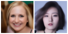
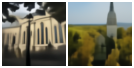
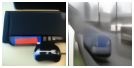
Figure 5: Interpolating between two inverted latent vectors and the generated results, with image at \(\alpha = 0\), image at \(\alpha = 1\), and the interpolation animation of intermediate \(\alpha\) values.

Suppose we have two images \(\mathbf{x}_1\) and \(\mathbf{x}_2\) and their respective inverted latent vector \(\mathbf{z}_1\) and \(\mathbf{z}_2\), we can interpolate \(\mathbf{x}_1\) and \(\mathbf{x}_2\) in image space by interpolating \(\mathbf{z}_1\) and \(\mathbf{z}_2\) in latent space. Particularly, we assume \(\mathbf{z} \sim \mathcal{N}(0, \mathbf{I})\), linear interpolation does not maintain the magnitude of \(\mathbf{z}\) (e.g., consider \(\mathbf{z}_1 = -\mathbf{z}_2\) as an extreme example), so we instead use spherical interpolation inspired by [1]. Given two latent vectors \(\mathbf{z}_1\) and \(\mathbf{z}_2\) and some \(\alpha \in [0, 1]\), where \(\alpha = 0\) produces \(\mathbf{z}_1\) and \(\alpha = 1\) produces \(\mathbf{z}_2\), we interpolate with

\[\theta = \arccos\left( \frac{\mathbf{z}_1 \cdot \mathbf{z}_2}{\| \mathbf{z}_1 \|_2 \| \mathbf{z}_2 \|_2} \right) \\ \hat{\mathbf{z}} = \frac{\sin((1 - \alpha) \theta)}{\sin(\theta)} \mathbf{z}_1 + \frac{\sin(\alpha \theta)}{\sin(\theta)} \mathbf{z}_2 ,\]

where \(\hat{\mathbf{z}}\) is the result of the interpolation that we can then use to generate the interpolated images.

def slerp(z_1, z_2, alpha):
    theta = torch.acos(torch.sum(z_1 * z_2) / (torch.norm(z_1) * torch.norm(z_2)))
    return torch.sin((1.0 - alpha) * theta) / torch.sin(theta) * z_1 + \
        torch.sin(alpha * theta) / torch.sin(theta) * z_2


def interpolation(z_1, z_2, diffusion, num_t_steps=10, num_alphas=100):
    x_mixes = []
    alphas = np.linspace(0.0, 1.0, num=num_alphas)
    for alpha in alphas:
        z_mix = slerp(z_1, z_2, alpha=alpha)
        x_mix = diffusion.sample(x=z_mix, sequence=False, num_t_steps=num_t_steps)[0]
        x_mixes.append(x_mix.detach().cpu())
    return x_mixes

Semantic Feature Editing

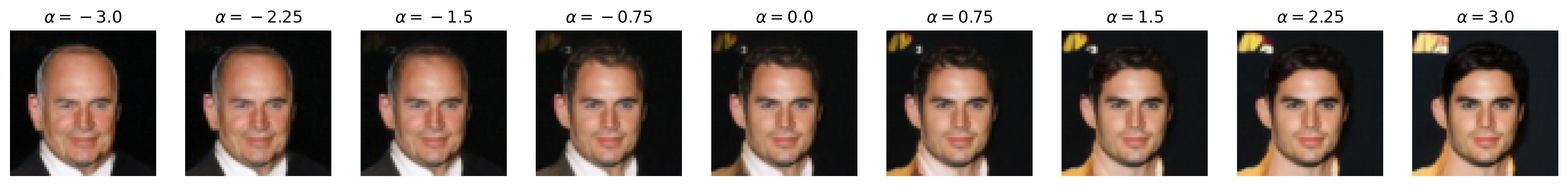
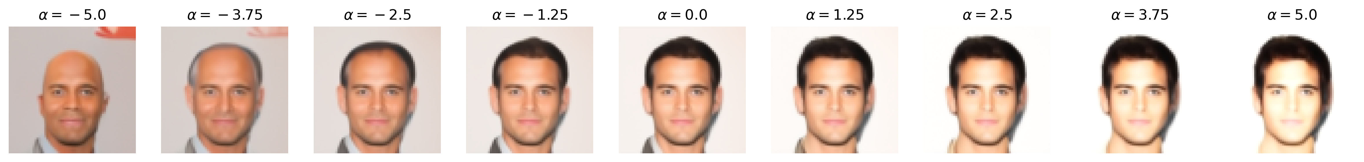
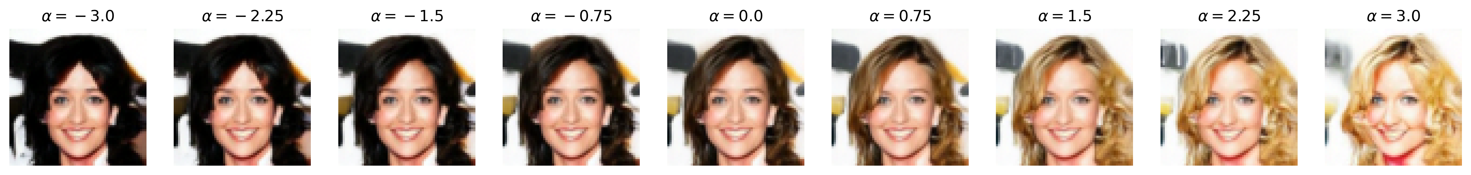
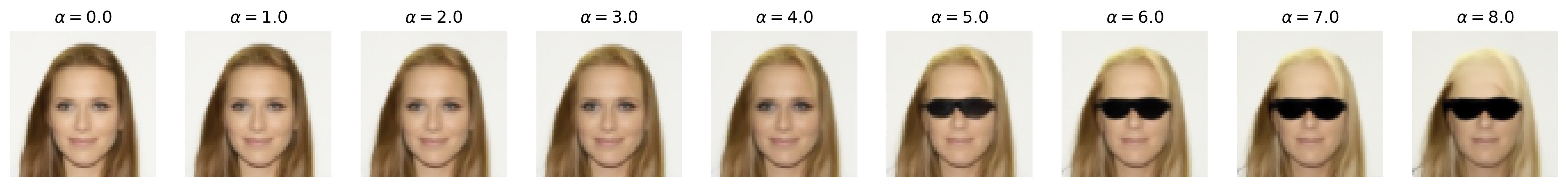
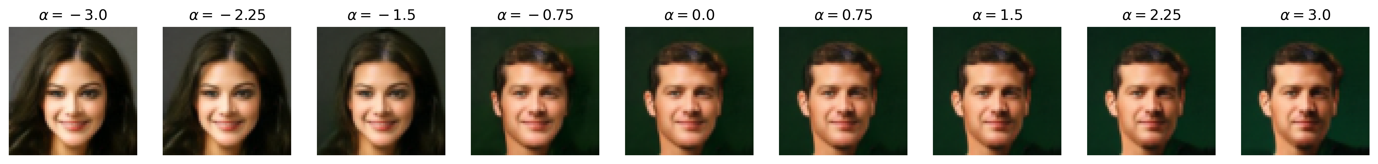
Attribute: Age Attribute: Attractiveness Attribute: Blonde hair Attribute: Eyeglasses Attribute: Masculinity Attribute: Smile

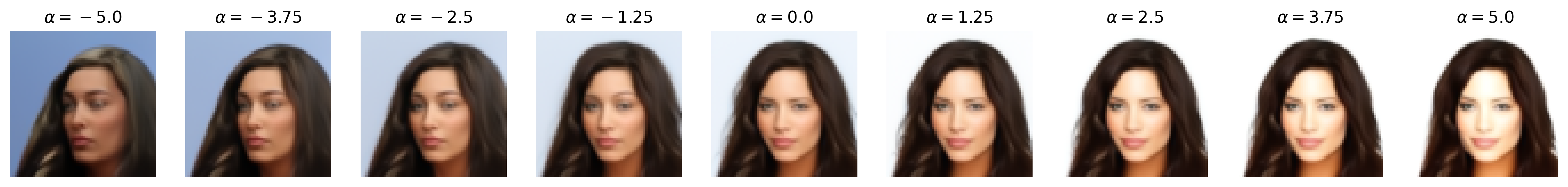
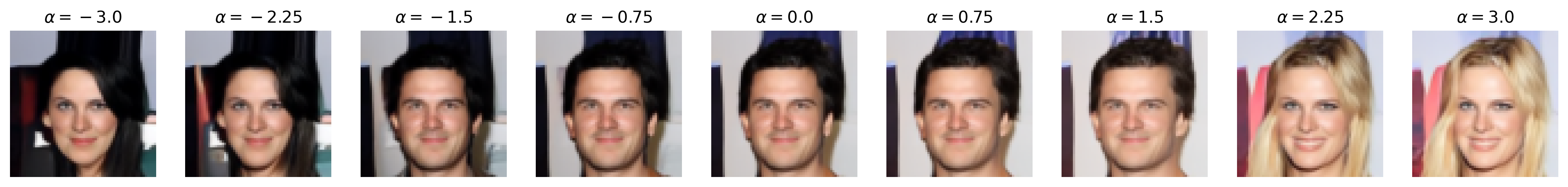
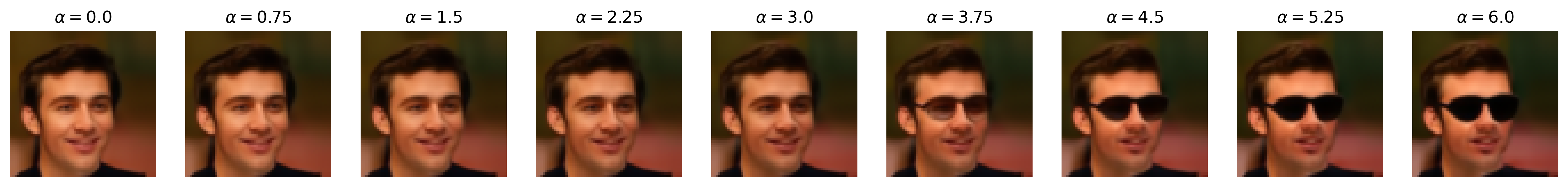
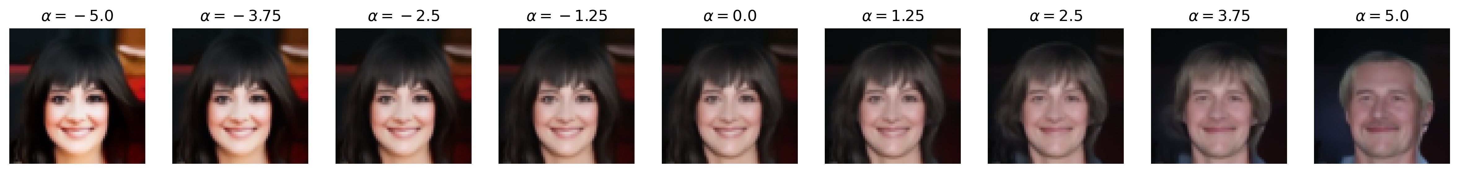
Figure 6: Semantic editing of generated faces for CelebA. Note that the ranges for \(\alpha\) is different for every sample as we manually try different values for each and pick the one which showcases the range of the editing the best.

We apply semantic feature editing on the CelebA dataset, as this is the only dataset we train DDIMs on which has extensive binary attribute annotations. There are \(40\) binary attributes, with notable ones including age, attractiveness (yikes), eyeglasses, masculinity, and smile. From the dataset, we train a multinomial classifier over the entire training dataset for all \(40\) binary attributes. For the multinomial classifier, we adopt the ResNet-20 architecture from [5] originally for CIFAR-10 classification, but we add an additional \(5 \times 5\) convolution with stride \(2\) to downsample the input images from \(64 \times 64\) to \(32 \times 32\), matching CIFAR-10. We use the same optimizer (SGD with Nesterov momentum) and learning rate scheduling (\(0.1\), drop by scale \(0.1\) at half-way and three-fourth point) as [5] and train for \(60000\) iterations.

Then, we pre-generate \(262144\) noise-image pairs. Note that, for this section, we set num_t_steps=50 for better generation detail (and that we are no longer backpropagating through the DDIM). We train a logistic regression classifier on each of the selected binary attributes we show above with these noise-image pairs, obtaining the direction vector (which is also the weight vector) \(\mathbf{w}\) that we normalize to obtain \(\mathbf{u}\). We train with SGD with Nesterov momentum and similar learning rate scheduling as above, with a weight decay of \(0.001\), and we train for \(10000\) iterations. (Note that, unlike [4], we do not pick the top and bottom \(10\)K images by binary attribute score and train the binary classifier on that, but we simply train on all \(262\)K images for simplicity. We also use logistic regression instead of a support vector machine, unlike [4], as our experiments with SVMs all did not work, likely due to not picking out the top and bottom \(10\)K images.) Then, we perform semantic image editing by pushing some \(\mathbf{z}\) with \(\mathbf{u}\) by \(\alpha\), as discussed in the Methods section.

Notice that, with many of these editing examples, the interpolated direction/attribute is not necessarily disentangled from other image features, which echoes [4] with semantic editing within the \(\mathcal{Z}\) space.

Visualizing the Decision Boundary

Age	Attractiveness	Blonde hair	Eyeglasses	Masculinity	Smile

Figure 7: Decision boundaries/direction vector \(\mathbf{u}\) of the binary attributes above, normalized to \([0, 1]\) for display.

Since the decision boundary or direction vector, \(\mathbf{u}\), is the same dimensions as the image by nature of the diffusion model, we can visualize it to see how it is pushing the noise latents to achieve semantic feature editing. Fascinatingly, we see that \(\mathbf{u}\) does indeed encode visual information, which is sensible, as the denoising inference process of diffusion models mean that we can add visual features we want directly to the noise latents to ‘guide’ the DDIM to generate the desired outputs. Although this can be done manually, the semantic feature editing method provides us a way to do so with a data-driven approach.

We see that the decision boundaries does indeed semantically correspond to the binary attributes themselves, as the one-to-one pixel-level mapping of the noise latent to the generated image makes \(\mathbf{u}\) easily visualized. For example, we can clearly see how the blonde hair vector adds a yellow ‘halo’ around the face which guides the DDIM to generate blonde hair, and how eyeglasses and smile have strongest effects around the eyes and the lips, respectively, which is sensible.

Importantly, the visualization of the decision boundary provides insight into the dataset (CelebA), specifically the bias inherently within the dataset. For example, we notice that the blonde hair vector seems to assume that the hair of the generated face is long, which is an effect we see with the feature editing results where those with short hair seems to ‘gain’ hair length when their hair becomes blonde. Similarly, the vectors for age and especially attractiveness display a rough face outline that looks more feminine than masculine, indicating not only an imbalance of these binary attributes between masculine and feminine faces (i.e., feminine faces are more likely to be labeled “young” or “attractive”). More broadly, since CelebA is a dataset of celebrities, we can argue that age and attractiveness are perhaps attributes more valued in female celebrities than male ones. We see this with the feature editing results as well, as age and attractiveness seems to be entangled with masculinity.

This sort of visualization shows one advantage of the DDIM latent space over the GAN latent space—interpretability. Even though the GAN latent space is arguably superior to the DDIM latent space in every way, with its lower dimensionality for easier computation, existence of more separated \(\mathcal{W}\) space with StyleGAN designs that provides coarse to fine control, and an inference process that requires just one forward propagation (and thus one backpropagation for most inversion techniques). However, the fact that the DDIM noise latent space is the same dimension as its image space, and that there is a direct spatial correspondence between the pixels in the noise latent space and that of the image space by the diffusion (denoising) process, means the noise latent space has great interpretability, as we have seen with the decision boundary visualization above.

Conclusion

We explore implementing and training a DDIM from scratch, utilizing its deterministic sampling process to probe the relationship between its latent noise space \(\mathcal{Z}\) and the image space \(\mathcal{X}\) by applying existing GAN inversion techniques to the DDIM. Particularly, we find the following.

1. Optimization-based inversion with the DDIM is possible and can produce relatively high-quality results, though currently it is limited to DDIM inferences with small num_t_steps as we must backpropagate through the model num_t_steps times.
2. Learning-based (and consequently hybrid) inversion with the DDIM is currently difficult, both due to the high memory requirements with larger num_t_steps (which can cause gradient vanishing) and that \(\mathcal{Z}\) is high-dimensional like \(\mathcal{X}\) making encoders difficult to train.
3. Interpolation between two noise latents leads to smooth visual interpolation in the image space for DDIMs, indicating that the latent space for diffusion models is smooth and meaningful, like that of GANs.
4. We can perform semantic feature editing by finding decision boundaries of binary attributes of images in the noise latent and changing the noise latent by the normal of the hyperplane. Due to the matching dimensions and spatial correspondence of \(\mathcal{Z}\) and \(\mathcal{X}\), we can visualize the decision boundary like an image, demonstrating the unique interpretability of the DDIM latent space.

The above shows the potential for research in manipulating the DDIM latent space directly, especially since the diffusion model can be conditioned in a variety of ways (e.g., class-condition, text-condition, and the recent ControlNet) in a variety of spaces (e.g., latent diffusion), which creates many latent spaces that can be manipulated in various ways.

Future Work

The following are some possible future directions based on the current project.

1. The current implementation of our optimization-based method solely minimizes the error within the image space. However, we can also minimize the error within the feature space, i.e., try to match the VGG/Inception features of the target and reconstruction. Though doing so generally leads to images that deviate in detail to the original, it reduces overfitting of the trained noise latent and thus makes interpolation and semantic editing smoother.
2. One of the biggest obstacles with learning-based (and consequently hybrid) inversion methods is the multiple forward (and thus backward) passes through the model. However, very recently OpenAI proposed consistency models, which, extremely simplified, is diffusion models that only require one forward pass [6]. In a way, the consistency model is similar to GANs with the generation process, but now it has the advantage of an interpretable latent space. It can be a potential direction for inversion.
3. There, in fact, already exists a method, called EDICT (Exact Diffusion Inversion via Coupled Transformations) which modifies the inference process of the DDIM with coupled transformations that allows near-exact inversion with results that are genuinely impressive. They also showed how using the DDIM inference process on Stable Diffusion to find the image noise latent and text latent, then only modifying the text latent, allows for semantic editing targeting the subject [7]. EDICT can potentially make the semantic feature editing methods easier as they provide exact inversion on unseen images.
4. The semantic face editing method is only a very small part of the bigger project, GenForce, which has a lot of GAN latent space manipulation methods (e.g., disentangling binary attributes via conditioning, better decision boundary computation with SVMs, better inversion methods, etc.) that can potentially be applied to DDIMs.

References

[1] Song, Jiaming, et al. “Denoising Diffusion Implicit Models.” International Conference on Learning Representations, 2021.

[2] Xia, Weihao, et al. “GAN Inversion: A Survey.” IEEE Transactions on Pattern Analysis & Machine Intelligence, 2022.

[3] Ho, Jonathan, et al. “Denoising Diffusion Probabilistic Models.” Advances in Neural Information Processing Systems, 2020, vol. 33, pp. 6840–6851.

[4] Shen, Yujun, et al. “Interpreting the Latent Space of GANs for Semantic Face Editing.” Proceedings of the IEEE/CVF Conference on Computer Vision and Pattern Recognition, 2020.

[5] He, Kaiming, et al. “Deep Residual Learning for Image Recognition.” Proceedings of the IEEE/CVF Conference on Computer Vision and Pattern Recognition, 2016.

Future Work References

[6] Song, Yang, et al. “Consistency Models.” arXiv:2303.01469, 2023.

[7] Wallace, Bram, et al. “EDICT: Exact Diffusion Inversion via Coupled Transformations.” arXiv:2211.12446, 2022.

Code Repository References

[1C] Original PyTorch implementation of DDIM
DDIM implementation from the original authors. I follow the code base closely for our implementation with slight changes, though I do not copy code and merely use their code as a vessel for understanding the paper. Particularly, the introduction section is entirely original by me and represents my ‘take’ on DDPMs and DDIMs after having implemented and trained both from scratch. The organization of the code modules is also changed to better fit my preference for ML repositories, particularly integration with Jupyter Notebook so I can experiment with the trained models.

[2C] Keras implementation of DDIM
Keras implementation of DDIM tested on Oxford Flowers102 dataset at a small scale trainable on my laptop. I took inspiration of some of their hyperparameter, criterion, and architecture design choices. Particularly, I inherited the use of \(L_1\) instead of \(L_2\) loss and the occasional batch normalization instead of group normalization for smaller networks and/or datasets with high detail.

[3C] The annotated diffusion model
The Hugging Face implementation and annotation of the DDPM. This is the original code I followed last quarter (when I was experimenting on my own) to get a basic understanding of DDPMs, and I partly based my code module organization and variable naming conventions on the blog post.